1. Introduction

The purpose of this technical note is to describe the physical parameterizations, numerical implementation, coding conventions and software architecture for the NCAR Weather Research and Forecasting model (WRF) hydrological modeling system, hereafter referred to as WRF-Hydro. The system is intended to be flexible and extensible and users are encouraged to develop, add and improve components to meet their application needs.

It is critical to understand that like the WRF atmospheric modeling system, the WRF-Hydro modeling system is not a singular ‘model’ per se but instead it is a modeling architecture that facilitates coupling of multiple alternative hydrological process representations. There are numerous (over 100) different configuration permutations possible in WRF-Hydro Version 5.4. Users need to become familiar with the concepts behind the processes within the various model options in order to optimally tailor the system for their particular research and application activities.

1.1 Brief History

The WRF-Hydro modeling system provides a means to couple hydrological model components to atmospheric models and other Earth System modeling architectures. The system is intended to be extensible and is built upon a modular Modern Fortran architecture. The code has also been parallelized for distributed memory parallel computing applications. Numerous options for terrestrial hydrologic routing physics are contained within Version 5.4 of WRF-Hydro but users are encouraged to add additional components to meet their research and application needs. The initial version of WRF-Hydro (originally called ‘Noah-distributed’ in 2003) included a distributed, 3-dimensional, variably-saturated surface and subsurface flow model previously referred to as ‘Noah-distributed’ for the underlying land surface model upon which the original code was based. Initially, the implementation of terrain routing and, subsequently, channel and reservoir routing functions into the 1-dimensional Noah land surface model was motivated by the need to account for increased complexity in land surface states and fluxes and to provide physically-consistent land surface flux and stream channel discharge information for hydrometeorological applications. The original implementation of the surface overland flow and subsurface saturated flow modules into the Noah land surface model are described by Gochis and Chen (2003). In that work, a simple subgrid disaggregation-aggregation procedure was employed as a means of mapping land surface hydrological conditions from a “coarsely” resolved land surface model grid to a much more finely resolved terrain routing grid capable of adequately resolving the dominant local landscape gradient features responsible for the gravitational redistribution of terrestrial moisture. Since then numerous improvements to the Noah-distributed model have occurred including optional selection for 2-dimensional (in \(x\) and \(y\)) or 1-dimensional (“steepest descent” or so-called “D8” methodologies) terrain routing, a 1-dimensional, grid-based, hydraulic routing model, a reservoir routing model, 2 reach-based hydrologic channel routing models, and a simple empirical baseflow estimation routine. In 2004, the entire modeling system, then referred to as the NCAR WRF-Hydro hydrological modeling extension package was coupled to the Weather Research and Forecasting (WRF) mesoscale meteorological model (Skamarock et al., 2005) thereby permitting a physics-based, fully coupled land surface hydrology-regional atmospheric modeling capability for use in hydrometeorological and hydroclimatological research and applications. The code has since been fully parallelized for high-performance computing applications. During late 2011 and 2012, the WRF-Hydro code underwent a major reconfiguration of its coding structures to facilitate greater and easier extensibility and upgradability with respect to the WRF model, other hydrological modeling components, and other Earth system modeling frameworks. Additional changes to the directory structure occurred during 2014-2015 to accommodate the coupling with the new Noah-MP land modeling system. Between 2015-2018, new capabilities were added to permit more generalized, user-defined mapping onto irregular objects, such as catchments or hydrologic response units. During 2018-2022, some of the modules underwent a code refactoring and automated testing capabilities were added. In 2024, the directory structure was again updated for consistency with modern software design practices and this user guide was ported to an interactive online format. As additional changes and enhancements to WRF-Hydro occur they will be documented in future versions of this document.

1.2 Model Description

WRF-Hydro has been developed to facilitate improved representations of terrestrial hydrologic processes related to the spatial redistribution of surface, subsurface and channel waters across the land surface and to facilitate coupling of hydrologic models with atmospheric models. Switch-activated modules in WRF-Hydro enable treatment of terrestrial hydrological physics, which have either been created or have been adapted from existing distributed hydrological models. The conceptual architecture for WRF-Hydro is shown in Figures 1.1 and 1.2 where WRF-Hydro exists as a coupling architecture (blue box) or “middle-ware” layer between weather and climate models and terrestrial hydrologic models and land data assimilation systems. WRF-Hydro can also operate in a standalone mode as a traditional land surface hydrologic modeling system.

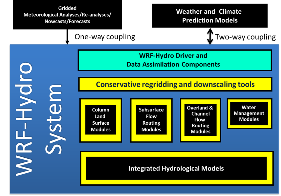
Figure 1.1. Generalized conceptual schematic of the WRF-Hydro architecture showing various categories of model components.

Figure 1.2. Model schematic illustrating where many existing atmosphere, land surface and hydrological model components could fit into the WRF-Hydro architecture. NOTE: Not all of these models are currently coupled into WRF-Hydro at this time. This schematic is meant to be illustrative. Components which are coupled have an asterisk (*) by their name.

WRF-Hydro is designed to enable improved simulation of land surface hydrology and energy states and fluxes at a fairly high spatial resolution (typically 1 km or less) using a variety of physics-based and conceptual approaches. As such, it is intended to be used as either a land surface model in both standalone (“uncoupled” or “offline”) mode and fully-coupled (to an atmospheric model) mode. Both time-evolving “forcing” and static input datasets are required for model operation. The exact specification of both forcing and static data depends greatly on the selection of model physics and component options to be used. The principal model physics options in WRF-Hydro include:

• 1-dimensional (vertical) land surface parameterization

• surface overland flow

• saturated subsurface flow

• channel routing

• reservoir routing

• conceptual/empirical baseflow

Both the Noah land surface and Noah-MP land surface model options are available for use in the current version of the WRF-Hydro. The rest of this document will focus on their implementation. Future versions will include other land surface model options.

Like nearly all current land surface models, the Noah and Noah-MP land surface parameterizations require a few basic meteorological forcing variables. Required meteorological forcing variables are listed in Table 1.1.

Table 1.1 Required input meteorological forcing variables for the Noah and Noah-MP LSMs

Variable	Units
Incoming shortwave radiation	\(W/m^2\)
Incoming longwave radiation	\(W/m^2\)
Specific humidity	\(kg/kg\)
Air temperature	\(K\)
Surface pressure	\(Pa\)
Near surface wind in the u - component	\(m/s\)
Near surface wind in the v-component	\(m/s\)
Liquid water precipitation rate	\(mm/s\)

[Different land surface models may require other or additional forcing variables or the specification of forcing variables in different units.]

When coupled to the WRF regional atmospheric model the meteorological forcing data is provided by the atmospheric model with a frequency dictated by the land surface model time-step specified in WRF. When run in a standalone mode, meteorological forcing data must be provided as gridded input time series. Further details on the preparation of forcing data for standalone WRF-Hydro execution is provided in 5.7 Specification of meteorological forcing data

External, third party, Geographic Information System (GIS) tools are used to delineate a stream channel network, open water (i.e., lake, reservoir, and ocean) grid cells and groundwater/baseflow basins. Water features are mapped onto the high-resolution terrain-routing grid and post-hoc consistency checks are performed to ensure consistency between the coarse-resolution Noah/Noah-MP land model grid and the fine-resolution terrain and channel routing grid.

The WRF-Hydro model components calculate fluxes of energy and moisture either back to the atmosphere or also, in the case of moisture fluxes, to stream and river channels and through reservoirs. Depending on the physics options selected, the primary output variables include but are not limited to those in the table below. Output variables and options are discussed in detail in 6. Description of Output Files from WRF-Hydro

Table 1.2 Primary Output data from WRF-Hydro

Variable	Units
Surface latent heat flux	\(W/m^2\)
Surface sensible heat flux	\(W/m^2\)
Ground heat flux	\(W/m^2\)
Ground surface and/or canopy skin temperature	\(K\)
Surface evaporation components (soil evaporation, transpiration, canopy water evaporation, snow sublimation and ponded water evaporation)	\(kg/m^2/s\)
Soil moisture	\(m^3/m^3\)
Soil temperature	\(K\)
Deep soil drainage	\(mm\)
Surface runoff	\(mm\)
Canopy moisture content	\(mm\)
Snow depth	\(m\)
Snow liquid water equivalent	\(mm\)
Stream channel inflow (optional with terrain routing)	\(mm\)
Channel flow rate (optional with channel routing)	\(m^3/s\)
Channel flow depth (optional with channel routing)	\(mm\)
Reservoir height and discharge (optional with channel and reservoir routing)	\(m\) and \(m^3/s\)

WRF-Hydro has been developed for Linux-based operating systems including small local clusters and high-performance computing systems. Additionally, the model code has also been ported to a selection of virtual machine environments (e.g. “containers”) to enable the use of small domain cases on many common desktop computing platforms (e.g. Windows and MacOS) and in the cloud. The parallel computing schema is provided in 2.3 Parallelization strategy. WRF-Hydro utilizes a combination of netCDF and flat ASCII file formats.

The majority of input and output is handled using the netCDF data format and the netCDF library is a requirement for running the model. Details on the software requirements are available online on the FAQs page of the website as well as in the How To Build & Run WRF-Hydro V5 in Standalone Mode document also available from https://ral.ucar.edu/projects/wrf_hydro.

WRF-Hydro is typically set up as a computationally-intensive modeling system. Simple small domains (e.g. 16 \(km^2\)) can be configured to run on a desktop platform. Large-domain model runs can require hundreds or thousands of processors. We recommend beginning with an example “test case” we supply at the WRF-Hydro website https://ral.ucar.edu/projects/wrf_hydro before moving to your region of interest, particularly if your region or domain is reasonably large.