3. Model Physics Description
This chapter describes the physics behind each of the modules in Version 5.4 of WRF-Hydro and the associated namelist options which are specified at “run time”.
3.1 Physics Overview
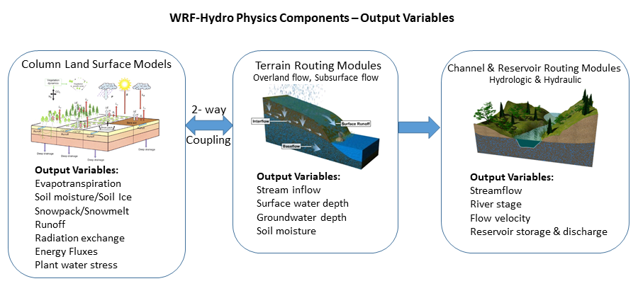
Figure 3.1. Conceptual diagram of WRF-Hydro physics components and relative outputs.
First, the 1-dimensional (1D) column land surface model calculates the vertical fluxes of energy (sensible and latent heat, net radiation) and moisture (canopy interception, infiltration, infiltration-excess, deep percolation) and soil thermal and moisture states. Infiltration excess, ponded water depth and soil moisture are subsequently disaggregated from the 1D LSM grid, typically of 1-4 km spatial resolution, to a high-resolution, typically 30-100 m, routing grid using a time-step weighted method (Gochis and Chen, 2003) and are passed to the subsurface and overland flow terrain-routing modules. In typical U.S. applications, land cover classifications for the 1D LSMs are provided by the USGS 24-type Land Use Land Cover product or MODIS Modified IGBP 20-category land cover product (see WRF/WPS documentation); soil classifications are provided by the 1-km STATSGO database (Miller and White, 1998); and soil hydraulic parameters that are mapped to the STATSGO soil classes are specified by the soil analysis of Cosby et al. (1984). Other land cover and soil type classification datasets can be used with WRF-Hydro but users are responsible for mapping those categories back to the same categories as used in the USGS or MODIS land cover and STATSGO soil type datasets. The WRF model pre-processing system (WPS) also provides a fairly comprehensive database of land surface data that can be used to set up the Noah and Noah-MP land surface models. It is possible to use other land cover and soils datasets, and more recently, data from the USGS National Land Cover Dataset (NLCD) and international soils datasets have been integrated into WRF-Hydro.
Then, subsurface lateral flow in WRF-Hydro is calculated prior to the routing of overland flow to allow exfiltration from fully saturated grid cells to be added to the infiltration excess calculated by the LSM. The method used to calculate the lateral flux of the saturated portion of the soil column is that of Wigmosta et al. (1994) and Wigmosta and Lettenmaier (1999), implemented in the Distributed Hydrology Soil Vegetation Model (DHSVM). It calculates a quasi-3D flow, which includes the effects of topography, saturated soil depth, and depth-varying saturated hydraulic conductivity values. Hydraulic gradients are approximated as the slope of the water table between adjacent grid cells in either the steepest descent or in both \(x\)- and \(y\)-directions. The flux of water from one cell to its down-gradient neighbor on each time-step is approximated as a steady-state solution. The subsurface flux occurs on the coarse grid of the LSM while overland flow occurs on the fine grid.
Next, WRF-Hydro calculates the water table depth according to the depth of the top of the saturated soil layer that is nearest to the surface. Typically, a minimum of four soil layers are used in a 2-meter soil column used in WRF-Hydro but this is not a strict requirement. Additional discretization permits improved resolution of a time-varying water table height and users may vary the number and thickness of soil layers in the model namelist described in the Appendices A3. Exceptions for Running WRF-Hydro with the Noah LSM, A4. Noah namelist.hrldas File with Description of Options, and A5. Noah-MP namelist.hrldas File with Description of Options.
Then, overland flow is defined. The fully unsteady, spatially explicit, diffusive wave formulation of Julien et al. (1995-CASC2D) with later modification by Ogden (1997) is the current option for representing overland flow, which is calculated when the depth of water on a model grid cell exceeds a specified retention depth. The diffusive wave equation accounts for backwater effects and allows for flow on adverse slopes (Ogden, 1997). As in Julien et al. (1995), the continuity equation for an overland flood wave is combined with the diffusive wave formulation of the momentum equation. Manning’s equation is used as the resistance formulation for momentum and requires specification of an overland flow roughness parameter. Values of the overland flow roughness coefficient used in WRF-Hydro were obtained from Vieux (2001) and were mapped to the existing land cover classifications provided by the USGS 24-type land-cover product of Loveland et al. (1995) and the MODIS 20-type land cover product, which are the same land cover classification datasets used in the 1D Noah/Noah-MP LSMs.
Additional modules have also been implemented to represent stream channel flow processes, lakes and reservoirs, and stream baseflow. In WRF-Hydro v5.4 inflow into the stream network and lake and reservoir objects is a one-way process. Overland flow reaching grid cells identified as ‘channel’ grid cells pass a portion of the surface water in excess of the local ponded water retention depth to the channel model. This current formulation implies that stream and lake inflow from the land surface is always positive to the stream or lake element. There is an optional channel loss formulation (Lahmers et al. 2019) where water can seep from the channel; note that this water becomes a sink term and is not returned to the soil or baseflow. Currently there are no channel or lake loss functions where water can move from channels or lakes back to the landscape. Channel flow in WRF-Hydro is represented by one of a few different user-selected methodologies described below. Water passing into and through lakes and reservoirs is routed using a simple level pool routing scheme. Baseflow to the stream network is represented using a conceptual catchment storage-discharge bucket model formulation (discussed below) which obtains “drainage” flow from the spatially-distributed landscape. Discharge from buckets is input directly into the stream using an empirically-derived storage-discharge relationship. If overland flow is active, the only water flowing into the buckets comes from soil drainage. This is because the overland flow scheme will pass water directly to the channel model. If overland flow is switched off and channel routing is still active, then surface infiltration excess water from the land model is collected over the pre-defined catchment and passed into the bucket as well. Each of these process options are enabled through the specification of options in the model namelist file.
3.2 Land model description: The community Noah and Noah-MP land surface models
Note
As of this writing, only the Noah and Noah-MP land surface models are supported within WRF-Hydro. CLM coupling is currently out-of-date and is not formally supported but is in the process of being updated. The NASA Land Information System (LIS) has been coupled with WRF-Hydro through the NUOPC framework and is supported under the NASA Land Coupler.
3.2.1 Noah Land Surface Model (deprecated support only)
The Noah land surface model is a community, 1-dimensional land surface model that simulates soil moisture (both liquid and frozen), soil temperature, skin temperature, snowpack depth, snowpack water equivalent, canopy water content and the energy flux and water flux terms at the Earth’s surface (Mitchell et al., 2002; Ek et al., 2003). The model has a long heritage, with legacy versions extensively tested and validated, most notably within the Project for Intercomparison of Land surface Parameterizations (PILPS), the Global Soil Wetness Project (Dirmeyer et al. 1999), and the Distributed Model Intercomparison Project (Smith, 2002). Mahrt and Pan (1984) and Pan and Mahrt (1987) developed the earliest predecessor to Noah at Oregon State University (OSU) during the mid-1980’s. The original OSU model calculated sensible and latent heat flux using a two-layer soil model and a simplified plant canopy model. Development and implementation of the Noah land model has been sustained through the community participation of various agency modeling groups and the university community (e.g. Chen et al., 2005). Ek et al. (2003) detail the numerous changes that have evolved since its inception including, a four layer soil representation (with soil layer thicknesses of 0.1, 0.3, 0.6 and 1.0 m), modifications to the canopy conductance formulation (Chen et al., 1996), bare soil evaporation and vegetation phenology (Betts et al., 1997), surface runoff and infiltration (Schaake et al., 1996), thermal roughness length treatment in the surface layer exchange coefficients (Chen et al., 1997a) and frozen soil processes (Koren et al., 1999). More recently refinements to the snow-surface energy budget calculation (Ek et al., 2003) and seasonal variability of the surface emissivity (Tewari et al., 2005) have been implemented.
The Noah land surface model has been tested extensively in both offline (e.g., Chen et al., 1996, 1997; Chen and Mitchell, 1999; Wood et al., 1998; Bowling et al., 2003) and coupled (e.g. Chen et el., 1997, Chen and Dudhia, 2001, Yucel et al., 1998; Angevine and Mitchell, 2001; and Marshall et al., 2002) modes. The most recent version of Noah is currently one of the operational LSM’s participating in the interagency NASA-NCEP real-time Land Data Assimilation System (LDAS, 2003, Mitchell et al., 2004 for details). Gridded versions of the Noah model are currently coupled to real-time weather forecasting models such as the National Center for Environmental Prediction (NCEP) North American Model (NAM), and the community WRF model. Users are referred to Ek et al. (2003) and earlier works for more detailed descriptions of the 1-dimensional land surface model physics of the Noah LSM.
Note
Support for the Noah Land Surface Model within WRF-Hydro is currently frozen at Noah version 3.6. Since the Noah LSM is not under active development by the community, WRF-Hydro is continuing to support Noah in deprecated mode only. Some new model features, such as the improved output routines, have not been setup to be backward compatible with Noah. Noah users should follow the guidelines in Appendix A2 for adapting the WRF-Hydro workflow to work with Noah.
3.2.2 Noah-MP Land Surface Model (recommended)
Noah-MP is a land surface model (LSM) using multiple options for key land-atmosphere interaction processes (Niu et al., 2011). Noah-MP was developed to improve upon some of the limitations of the Noah LSM (Koren et al., 1999; Ek et al., 2003). Specifically, Noah-MP contains a separate vegetation canopy defined by a canopy top and bottom, crown radius, and leaves with prescribed dimensions, orientation, density, and radiometric properties. The canopy employs a two-stream radiation transfer approach along with shading effects necessary to achieve proper surface energy and water transfer processes including under-canopy snow processes (Dickinson, 1983; Niu and Yang, 2004). Noah-MP contains a multi-layer snow pack with liquid water storage and melt/refreeze capability and a snow-interception model describing loading/unloading, melt/refreeze capability, and sublimation of canopy-intercepted snow (Yang and Niu 2003; Niu and Yang 2004). Multiple options are available for surface water infiltration and runoff and groundwater transfer and storage including water table depth to an unconfined aquifer (Niu et al., 2007) as well as options for different snow processes such as snow albedo.
The Noah-MP land surface model can be executed by prescribing both the horizontal and vertical density of vegetation using either ground- or satellite-based observations. Another available option is for prognostic vegetation growth that combines a Ball-Berry photosynthesis-based stomatal resistance (Ball et al., 1987) with a dynamic vegetation model (Dickinson et al. 1998) that allocates carbon to various parts of vegetation (leaf, stem, wood and root) and soil carbon pools (fast and slow). The model is capable of distinguishing between \(C_3\) and \(C_4\) photosynthesis pathways and defines vegetation-specific parameters for plant photosynthesis and respiration.
In addition to the three-layer snow model in NoahMP, WRF-Hydro also supports optionally running the Crocus snowpack model within NoahMP for glacial representation. For details on using this option, please see Appendix 16.
The Noah-MP version in WRF-Hydro also includes an option for adjusting
infiltration vs. surface runoff partitioning as a function of impervious
surface cover. The default Noah-MP behavior is to set a very narrow range
of soil water holding capacity for cells classified as urban. This has the
effect of generating more runoff, but also results in very wet cells
that may or may not be appropriate for your application. The new physics setting
(IMPERV_OPTION in namelist.hrldas) includes 4 options:
Option 0 (no adjustment): Urban cells will be treated the same as all other cells and will use the provided soil and surface parameters to calculate partitoning between infiltration and surface runoff.
Option 1 (total): If spatially distributed parameters are active (
SPATIAL_SOIL=1on code compile), the model will expect an impervious fraction grid (imperv) to be included in the soil_properties.nc file. The model will use this fractional value to automatically partition that fraction (imperv) of effective precipitation reaching the surface to direct surface runoff. The rest (1-imperv) will be available for infiltration. If spatially distributed parameters are not active (SPATIAL_SOIL=0on code compile), the model will use theIMPERV_URBANvalue from MPTABLE.TBL for impervious fraction for all urban cells.Option 2 (Alley&Veenhuis): Similar to Option 1, with the modification that the provided impervious fraction will be adjusted to account for local capture of some runoff to adjacent green spaces. This adjustment uses an empirical formulation derived in Alley & Veenhuis (1983, https://doi.org/10.1061/(ASCE)0733-9429(1983)109:2(313) ). In the future we plan to test options that derive an adjustment factor based on impervious connectivity or other local (sub-grid) conditions.
Option 9 (original formulation): This reverts back to the original Noah-MP configuration where soil water holding capacity is adjusted for urban cells and impervious fraction is not used.
Note
The Noah-MP code within WRF-Hydro has some additional features that were added specifically for WRF-Hydro hydrologic applications, such as spatially distributed parameters and impervious surface runoff treatment, so it does not exactly track the Noah-MP standalone code releases. Standalone Noah-MP model code was recently modernized for modularity and accessibility (He et al. 2023). Support for this refactored version of the Noah-MP model is currently in development and will be included in a future WRF-Hydro release.
3.3 Spatial Transformations
The WRF-Hydro system has the ability to execute a number of physical process executions (e.g. column physics, routing processes, reservoir fluxes) on different spatial frameworks (e.g. regular grids, catchments, river channel vectors, reservoir polygons, etc). This means that spatial transformations between differing spatial elements has become a critical part of the overall modeling process. Starting in v5.0 of WRF-Hydro, increased support has been developed to aid in the mapping between differing spatial frameworks. Section 3.3.1 describes the spatial transformation process which relies on regular, rectilinear grid-to-grid mapping using a simplified integer linear multiple aggregation/disaggregation scheme. This basic scheme has been utilized in WRF-Hydro since its creation as it was described in Gochis and Chen, 2003.
Section 3.3.2 describes new spatial transformation methods that have been developed and are currently supported in v5.0 and beyond and, more specifically, in the NOAA National Water Model (NWM). Those user-defined transformations rely on the pre-processing development and specification of interpolation or mapping weights which must be read into the model. As development continues future versions will provide more options and flexibility for spatial transformations using similar user-defined methodologies.
3.3.1 Subgrid disaggregation-aggregation
This section details the implementation of a subgrid aggregation/disaggregation scheme in WRF-Hydro. The disaggregation-aggregation routines are activated when routing of either overland flow or subsurface flow is active and the specified routing grid increment is different from that of the land surface model grid. Routing in WRF-Hydro is “switch-activated” through the declaration of parameter options in the primary model namelist file hydro.namelist which are described in Appendix A5. Noah-MP namelist.hrldas File with Description of Options
In WRF-Hydro subgrid aggregation/disaggregation is used to represent overland and subsurface flow processes on grid scales much finer than the native land surface model grid. Hence, only routing is represented within a subgrid framework. It is possible to run both the land surface model and the routing model components on the same grid. This effectively means that the aggregation factor between the grids has a value of 1.0. This following section describes the aggregation/disaggregation methodology in the context of a “subgrid” routing implementation.
In WRF-Hydro the routing portions of the code have been structured so that it is simple to perform both surface and subsurface routing calculations on grid cells that potentially differ from the native land surface model grid sizes provided that each land surface model grid cell is divided into integer portions for routing. Hence routing calculations can be performed on comparatively high-resolution land surfaces (e.g., a 25 \(m\) digital elevation model) while the native land surface model can be run at much larger (e.g., 1 \(km\)) grid sizes. (In this example, the integer multiple of disaggregation in this example would be equal to 40.) This capability adds considerable flexibility in the implementation of WRF-Hydro. However, it is well recognized that surface hydrological responses exhibit strongly scale-dependent behavior such that simulations at different scales, run with the same model forcing, may yield quite different results.
The aggregation/disaggregation routines are currently activated by
specifying either the overland flow or subsurface flow routing options
in the model namelist file and prescribing terrain grid domain file
dimensions (IXRT, JXRT) which differ from the land surface model domain
file dimensions (IX, JX). Additionally, the model sub-grid size (DXRT),
the routing time-step (DTRT), and the integer divisor (AGGFACTRT), which
determines how the aggregation/disaggregation routines will divide up a
native model grid square, all need to be specified in the model
\(hydro.namelist\) file.
If IXRT=IX, JXRT=JX and AGGFACTRT=1 the aggregation/disaggregation
schemes will be activated but will not yield any effective changes in
the model resolution between the land surface model grid and the terrain
routing grid. Specifying different values for IXRT, JXRT and AGGFACTRT≠1
will yield effective changes in model resolution between the land model
and terrain routing grids. As described in the Surface Overland Flow
Routing section 3.5, DXRT and DTRT
must always be specified in accordance with the routing grid even if
they are the same as the native land surface model grid.
The disaggregation/aggregation routines are implemented in WRF-Hydro as
two separate spatial loops that are executed after the main land surface
model loop. The disaggregation loop is run prior to routing of saturated
subsurface and surface water. The main purpose of the disaggregation
loop is to divide up specific hydrologic state variables from the land
surface model grid square into integer portions as specified by
AGGFACTRT. An example disaggregation (where AGGFACTRT=4) is given in
Figure 3.2.
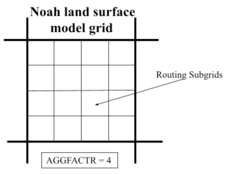
Figure 3.2 Example of the routing sub-grid implementation within the regular land surface model grid for an aggregation factor = 4.
Four model variables are required to be disaggregated for higher resolution routing calculations:
\(SMCMAX\) - maximum soil moisture content for each soil type
\(SMCREF\) - reference soil moisture content (field capacity) for each soil type
\(INFXS\) - infiltration excess
\(LKSAT\) - lateral saturated conductivity for each soil type
\(SMC\) - soil moisture content for each soil layer
In the model code, fine-grid values bearing the same name as these with
an “RT” extension are created for each native land surface model grid
cell (e.g. INFXSRT vs INFXS).
To preserve the structure of the spatial variability of soil moisture content on the sub-grid from one model time step to the next, simple, linear sub-grid weighting factors are assigned. These values indicate the fraction of the total land surface model grid value that is partitioned to each sub-grid pixel. After disaggregation, the routing schemes are executed using the fine-grid values.
Following execution of the routing schemes the fine-grid values are
aggregated back to the native land surface model grid. The aggregation
procedure used is a simple linear average of the fine-grid components.
For example the aggregation of surface head (SFHEAD) from the fine grid
to the native land surface model grid would be:
\({SFHEAD}_{i,j}\ = \ \frac{\Sigma\Sigma\ {SFHEADRT}_{irt,jrt}}{AGGFACTRT^2}\) (3.0)
where, \(i_{rt}\) and \(j_{rt}\) are the indices of all of the grid cells residing within the native land model grid cell \(i\),\(j\). The following variables are aggregated and, where applicable, update land surface model variable values:
SFHEAD - surface head (or, equivalently, depth of ponded water)SMC - soil moisture content for each soil layer
These updated values are then used on the next iteration of the land surface model.
3.3.2 User-Defined Mapping
The emergence of hydrologic models, like WRF-Hydro, that are capable of running on gridded as well as vector-based processing units requires generic tools for processing input and output data as well as methods for transferring data between models. Such a spatial transformation is currently utilized when mapping between model grids and catchments in the WRF-Hydro/National Water Model (NWM) system. In the NWM, selected model fluxes are mapped from WRF-Hydro model grids onto the NHDPlus catchment polygon and river vector network framework. The GIS pre-processing framework described here allows for fairly generalized geometric relationships between features to be characterized and for parameters to be summarized for any discrete unit of geography.
3.3.3 Data Remapping for Hydrological Applications
A common task in hydrologic modeling is to regrid or aggregate data from one unit of analysis to another. Frequently, atmospheric model data variables such as temperature and precipitation may be produced on a rectilinear model grid while the hydrologic unit of analysis may be a catchment Hydrologic Response Unit (cHRU), defined using a closed polygon and derived from a hydrography dataset or terrain processing application. Often, cHRU-level parameters must be derived from data on a grid. Depending on the difference between the scale of the gridded and feature data, simple interpolation schemes such as nearest neighbor may introduce significant error when estimating data at the cHRU scale. Other GIS analysis methods such as zonal statistics require resampling of the gridded and/or feature data and limited control over the common analysis grid resolution, which may also introduce significant error. Area-weighted grid statistics provide a robust and potentially conservative method for transferring data from one or multiple features to another. In the case of runoff calculated from a land surface model grid, the runoff should be conservatively transferred between the grid and the cHRU, such that the runoff volume is conserved.
The correspondence between polygons and grid cells need only be generated once for any grid/polygon collection. The correspondence file that is output from the tool stores all necessary information for translating data between the datasets in either direction.
There are a variety of useful regridding and spatial analysis tools available for use in the hydrologic and atmospheric sciences. Many regridding utilities exist that are able to either characterize and store the relationship between grid features and polygons or perform regridding from one grid to another. The Earth System Modeling Framework (ESMF) offers high performance computing (HPC) software for building and coupling weather, climate, and related models. ESMF provides the ESMF_RegridWeightGen utility for parallel generation of interpolation weights between two grid files in netCDF format. These utilities will work for structured (rectilinear) and unstructured grids. The ESMF_RegridWeightGen tool since can be accessed through python (through ESMPy) and the NCAR Command Language (NCL, deprecated). Another commonly used tool in the atmospheric sciences are the Climate Data Operators (CDO), which offer 1st and 2nd- order conservative regridding (remapcon, remapcon2) and regrid weight generation (gencon, gencon2) based on the work of Jones (1999). All of the above-mentioned utilities require SCRIP grid description files to perform the remapping. The SCRIP standard format for correspondence stores geometry information for regridding, while the tools mentioned here store just the spatial weights. Thus, WRF-Hydro spatial correspondence files are more generic, with compact file sizes, and may be used for non-gridded data.
The WRF-Hydro geospatial pre-processing toolkit includes a script that quantifies the polygon to polygon correspondence between geometries in two separate features (grid cells represented by polygons and basins represented by polygons). This correspondence is stored in a netCDF format file that contains the spatial weights and identification of all polygons from one input shapefile that intersect each polygon in another input shapefile. The storage of correspondence information between one dataset and another allows for many types of regridding and spatial interpolation between the spatial datasets. This file needs only to be derived once between any two sets of polygons, and the correspondence file can be used to regrid variables between those spatial datasets. This is useful if multiple variables must be regridded, or a single variable across many timesteps. As long as the grids do not change in space or time, the relationship between all features will remain constant, and the correspondence file may be used to regrid data between them.
There are uses for this utility that range outside of the hydrological sciences, and this utility may be of broader interest to the geospatial community. Although interpolation packages exist, this method allows for storage of the correspondence information for future use in a small-file size. Users wanting to create custom spatial weight interpolation files for WRF-Hydro need to refer to the WRF-Hydro GIS Pre-processing Toolkit and documentation. For reference, variable descriptions of the contents of the spatial weights file is located in A13. Spatial weights input file variable description.
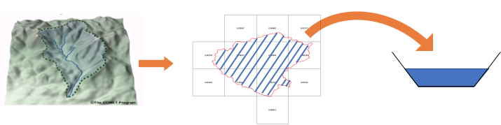
Figure 3.3. An illustration of implementing user-defined mapping to translate from gridded fluxes and states to aggregated catchment fluxes and states, which can be passed into, for example, vector-based channel routing modules.
3.4 Subsurface Routing
Subsurface lateral flow is calculated prior to the routing of overland flow. This is because exfiltration from a supersaturated soil column is added to infiltration excess from the land surface model, which ultimately updates the value of surface head prior to routing of overland flow. A supersaturated soil column is defined as a soil column that possesses a positive subsurface moisture flux which when added to the existing soil water content is in excess of the total soil water holding capacity of the entire soil column. Figure 3.4 illustrates the lateral flux and exfiltration processes in WRF-Hydro.
In the current default implementation of WRF-Hydro with the Noah and
Noah-MP land surface models, there are four soil layers. The depth of
the soil layers in WRF-Hydro can be manually specified in the model
namelist file under the ZSOIL variable. Users must be aware that, in
the present version of WRF-Hydro, total soil column depth and individual
soil layer thicknesses are constant throughout the entire model domain.
Future versions under development are relaxing this constraint. However,
the model is capable of using a different distribution of soil column
layer depths and these simply need to be specified in the model namelist
file. Assuming a 2-m soil profile the default soil layer depths (and
associated water table depths) are specified in Table 3.1.
Layer |
Soil Thickness (mm) |
Z (depth to top of layer) (mm) |
|---|---|---|
1 |
100 |
0 |
2 |
300 |
100 |
3 |
600 |
400 |
4 |
1000 |
1000 |
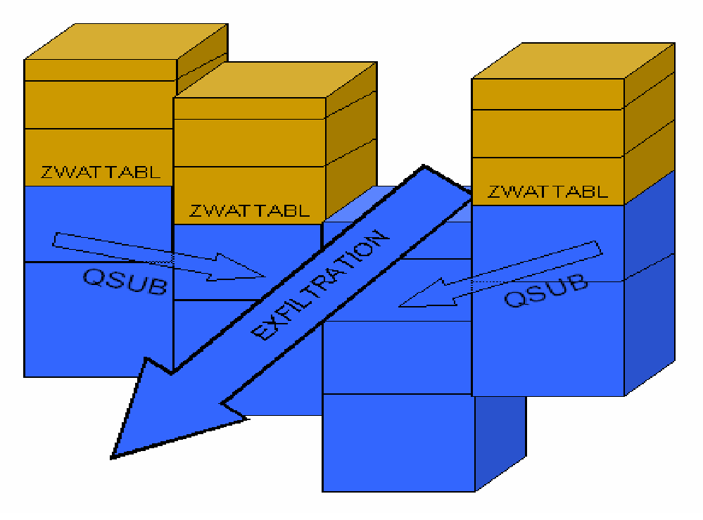
Figure 3.4 Conceptualization of saturated subsurface flow components.
The method used to calculate the lateral flow of saturated soil moisture employs a quasi three-dimensional flow representation, which include the effects of topography, saturated soil depth (in this case layers), and saturated hydraulic conductivity. Hydraulic gradients are approximated as the slope of the water table between adjacent grid cells in the x- and y-directions or in an eight direction (D8) steepest descent methodology that is specified by the user in the model namelist. In each cell, the flux of water from one cell to its down-gradient neighbor on each timestep is approximated as a steady-state solution. The looping structure through the model grid performs flux calculations separately in the x- and y-directions for the 2-dimensional routing option or simply along the steepest D8 pathway.
Using Dupuit-Forchheimer assumptions the rate of saturated subsurface flow at time \(t\) can be calculated as:
where, \(q_{i,j}\) is the flow rate from cell \((i,j)\), \(T_{i,j}\) is the transmissivity of cell \((i,j)\), \(\beta_{i,j}\) is the water table slope and \(w_{i,j}\) is the width of the cell which is fixed for a regular grid. \(\beta_{i,j}\) is calculated as the difference in water table depths between two adjacent grid cells divided by the grid spacing. The method by which the water table depth is determined is provided below. Transmissivity is a power law function of saturated hydraulic conductivity (\(Ksat_{i,j}\)) and soil thickness (\(D_{i,j}\)) given by:
where, \(z_{i,j}\) is the depth to the water table. \(n_{i,j}\) in Eq. (3.2) is defined as the local power law exponent and is a tunable parameter that dictates the rate of decay of \(Ksat_{i,j}\) with depth (\(n_{i,j}\) has a default value of 1.0 or can be specified as “NEXP” in hydro2dtbl.nc). When Eq. (3.2) is substituted into Eq. (3.1) the flow rate from cell \((i,j)\) to its neighbor in the \(x\)-direction can be expressed as:
where,
This calculation is repeated for the y-direction when using the two-dimensional routing method. The net lateral flow of saturated subsurface moisture (\(Q_{net}\)) for cell \((i,j)\) then becomes:
The mass balance for each cell on a model time step (\(\Delta t\)) can then be calculated in terms of the change in depth to the water table (\(\Delta z\)):
where, \(\phi\) is the soil porosity, \(R\) is the soil column recharge rate from infiltration or deep subsurface injection and A is the grid cell area. In WRF-Hydro, \(R\), is implicitly accounted for during the land surface model integration as infiltration and subsequent soil moisture increase. Assuming there is no deep soil injection of moisture (i.e. pressure driven flow from below the lowest soil layer), \(R\), in WRF-Hydro is set equal to 0.
The methodology outlined in Equations 3.2 thru 3.7 has no explicit information on soil layer structure, as the method treats the soil as a single homogeneous column (with an assumed exponential decay of saturated hydraulic conductivity). Therefore, changes in water table depth (\(\Delta z\)) need to be remapped to the land surface model soil layers. WRF-Hydro specifies the water table depth according to the depth of the top of the highest (i.e. nearest to the surface) saturated layer. The residual saturated water above the uppermost, saturated soil layer is then added to the overall soil water content of the overlying unsaturated layer. This computational structure requires accounting steps to be performed prior to calculating \(Q_{net}\).
Given the timescale for groundwater movement and limitations in the
model structure there is significant uncertainty in the time it takes to
properly spin-up groundwater systems. The main things to consider
include 1) the specified depth of soil and number and thickness of the
soil vertical layers and 2) the prescription of the model bottom
boundary condition. Typically, for simulations with deep soil profiles
(e.g. > 10 \(m\)) the bottom boundary condition is set to a ‘no-flow’
boundary (SLOPE_DATA = 0.0 in the GENPARM.TBL parameter file
or slope = 0.0 in the soil_properties.nc spatially distributed
parameter file). See Appendices A6. WRF-Hydro hydro.namelist File with Description of Options and A7. Static input files for WRF-Hydro for a
description of GENPARM.TBL and soil_properties.nc.
Note
Currently subsurface routing is only supported in the steepest slope (D8) formulation. The 2-dimensional solution will be reactivated in a future release.
Relevant code modules:
Routing/Noah_distr_routing_subsurface.F90
Relevant namelist options:
hydro.namelist:
SUBRTSWCRT- Switch to activate subsurface flow routing.DXRT- Specification of the routing grid cell spacingAGGFACTR- Subgrid aggregation factor, defined as the ratio of the subgrid resolution to the native land model resolution
namelist.hrldas:
NOAH_TIMESTEP- Subsurface routing operates on the LSM timestep
Relevant domain and parameter files/variables:
TOPOGRAPHYin Fulldom_hires.nc - Terrain grid or Digital Elevation Model (DEM). Note: this grid may be provided at resolutions equal to or finer than the native land model resolution.LKSATFACin Fulldom_hires.nc - Multiplier on saturated hydraulic conductivity in lateral flow direction.SATDK,SMCMAX,SMCREFin HYDRO.TBL or hydro2dtbl.nc - Soil properties (saturated hydraulic conductivity, porosity, field capacity) used in lateral flow routing.NEXPin hydro2dtbl.nc - Local power law exponent that dictates the rate of decay of saturated hydraulic conductivity with depth.
3.5 Surface Overland Flow Routing
Overland flow in WRF-Hydro is calculated using a fully-unsteady, explicit, finite-difference, diffusive wave formulation similar to that of Julien et al. (1995) and Ogden et al. (1997). The diffusive wave equation, while slightly more complicated, is, under some conditions, superior to the simpler and more traditionally used kinematic wave equation, because it accounts for backwater effects and allows for flow on adverse slopes. The overland flow routine described below can be implemented in either a 2-dimensional (x and y direction) or 1-dimension (steepest descent or “D8”) method. While the 2-dimensional method may provide a more accurate depiction of water movement across some complex surfaces it is more expensive in terms of computational time compared with the 1-dimensional method. While the physics of both methods are identical we have presented the formulation of the flow in equation form below using the 2-dimensional methodology.

Figure 3.5: Conceptual representation of terrain elements. Flow is routed across terrain elements until it intersects a “channel” grid cell indicated by the blue line where it becomes “in-flow” to the stream channel network.
The diffusive wave formulation is a simplification of the more general St. Venant equations of continuity and momentum for a shallow water wave. The two-dimensional continuity equation for a flood wave flowing over the land surface is:
where, \(h\) is the surface flow depth; \(q_x\) and \(q_y\) are the unit discharges in the \(x\)- and \(y\)-directions, respectively; and \(i_e\) is the infiltration excess. The momentum equation used in the diffusive wave formulation for the \(x\)-dimension is:
where, \(S_fx\) is the friction slope (or slope of the energy grade line) in the x-direction, \(S_ox\) is the terrain slope in the \(x\)-direction and \(\partial h/\partial x\) is the change in depth of the water surface above the land surface in the \(x\)-direction.
In the 2-dimensional option, flow across the terrain grid is calculated first in the \(x\)- then in the \(y\)-direction. In order to solve Eq. 3.8 values for \(q_x\) and \(q_y\) are required. In most hydrological models they are typically calculated by the use of a resistance equation such as Manning’s equation or the Chezy equation, which incorporates the expression for momentum losses given in Eq. 3.9. In WRF-Hydro, a form of Manning’s equation is implemented:
where,
where, \(n_{OV}\) is the roughness coefficient of the land surface and is a tunable parameter and \(\beta\) is a unit-dependent coefficient expressed here for SI units.
The overland flow formulation has been used effectively at fine terrain scales ranging from 30-300 \(m\). There has not been rigorous testing to date, in WRF-Hydro, at larger length-scales (> 300 \(m\)). This is due to the fact that typical overland flood waves possess length scales much smaller than 1 \(km\). Micro-topography can also influence the behavior of a flood wave. Correspondingly, at larger grid sizes (e.g. > 300 \(m\)) there will be poor resolution of the flood wave and the small-scale features that affect it. Also, at coarser resolutions, terrain slopes between grid cells are lower due to an effective smoothing of topography as grid size resolution is decreased. Each of these features will degrade the performance of dynamic flood wave models to accurately simulate overland flow processes. Hence, it is generally considered that finer resolutions yield superior results.
The selected model time step is directly tied to the grid resolution. In order to prevent numerical diffusion of a simulated flood wave (where numerical diffusion is the artificial dissipation and dispersion of a flood wave) a proper time step must be selected to match the selected grid size. This match is dependent upon the assumed wave speed or celerity (\(c\)). The Courant Number, \(C_n = c(\Delta t/\Delta x)\), should be close to 1.0 in order to prevent numerical diffusion. The value of the \(C_n\) also affects the stability of the routing routine such that values of \(C_n\) should always be less than 1.0. Therefore the following model time steps are suggested as a function of model grid size as shown in Table 3.2.
X (\(m\)) |
T (\(s\)) |
|---|---|
30 |
2 |
100 |
6 |
250 |
15 |
500 |
30 |
WRF-Hydro also includes an impervious surface adjustment option for overland routing. If this
scheme is activated (imperv_adj = 0 in hydro.namelist) then the overland roughness
Manning’s coefficient and maximum retention depth are adjusted based on the impervious fraction
provided as IMPERVFRAC in Fulldom_hires.nc. Specifically, maximum retention depth
is multiplied by (1 - IMPERVFRAC) (so smaller values for higher imperviousness). Manning’s
roughness for overland routing is scaled based on a linear weighting of smoothness
(1/roughness, see Liong et al. 1989) and assuming a roughness of 0.02 for impervious and native
cell roughness for pervious:
OVROUGHRT = 1 / ((1/0.02)*impervfrac + (1/OVROUGHRT)*(1-impervfrac))
Relevant code modules:
Routing/Noah_distr_routing_overland.F90
Relevant namelist options:
\(hydro.namelist\):
OVRTSWCRT- Switch to activate overland flow routing.DXRT- Specification of the routing grid cell spacingAGGFACTR- Subgrid aggregation factor, defined as the ratio of the subgrid resolution to the native land model resolutionDTRT_TER- Overland routing grid time steprt_option- Overland flow routing option (steepest descent or 2-dimensional)
Relevant domain and parameter files/variables:
TOPOGRAPHYin Fulldom_hires.nc - Terrain grid or Digital Elevation Model (DEM). Note: this grid may be provided at resolutions equal to or finer than the native land model resolution.RETDEPRTFACin Fulldom_hires.nc - Multiplier on maximum retention depth before flow is routed as overland flow.OVROUGHRTFACin Fulldom_hires.nc - Multiplier on Manning’s roughness for overland flow.OV_ROUGHin HYDRO.TBL orOV_ROUGH2Din hydro2dtbl.nc - Manning’s roughness for overland flow (by default a function of land use type).
3.6 Channel Routing
There are multiple channel routing algorithms available in version 5.4 of WRF-Hydro. These algorithms operate either on the resolution of the fine grid (gridded routing) or on a vectorized network of channel reaches (linked routing, also referred to as reach-based routing), which maps the fine grid to the vector network (Figure 3.6). The following section describes the routing methods and their implementation in the WRF-Hydro model code.
In general, inflow to the channel is based on a mass balance calculation, where the channel routes water when the ponded water depth (or surface head, \(SFCHEADRT\)) of the channel grid cells exceeds a predefined retention depth (\(RETDEPRT\)). As described in Section 3.5, the depth of surface head on any grid cell is a combination of the local infiltration excess, the amount of water flowing onto the grid cell from overland flow, and exfiltration from groundwater flow. The quantity of surface head in excess of the retention depth is accumulated as stream channel inflow and is effectively “discharged” to the channel routing routine (described below). In the current code, \(RETDEPRT\) is hard-coded to 5mm for channel pixels to encourage more local infiltration near the river channel leading to wetter soils that better emulate riparian conditions. Values of “channel inflow” are accumulated on the channel grid and can be output for visualization and analysis (see Section 6 for a description of model outputs).
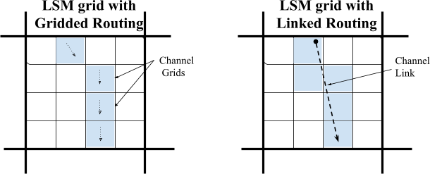
Figure 3.6 Channel routing via the high resolution grid (left) or on a vector/link network (right).
The channel routing module module_channel_routing.F90 allows for the one-dimensional, distributed routing of streamflow across the domain. An optional, switch-activated, level-pool lake/reservoir algorithm is also available and is described below in Sections 3.7 and 3.8. Within each channel grid cell there is an assumed channel reach of trapezoidal geometry as depicted in Figure 3.7. Channel parameters side slope (\(z\)), bottom width (\(B_w\)) and roughness (\(n\)) are currently prescribed as functions of Strahler stream order for defaults. Details on how each routing method reads these parameters are specified in the subsections below.
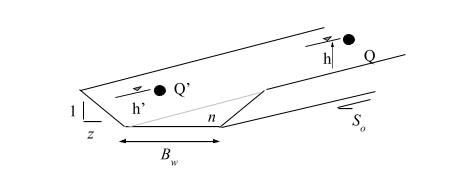
Figure 3.7 Schematic of Channel Routing Terms
Channel Slope |
\(S_o\) |
Channel Length |
\(\Delta x\) (\(m\)) |
Channel side slope |
\(z\) (\(m\)) |
Constant bottom width |
\(B_w\) (\(m\)) |
Manning’s roughness coefficient |
(\(n\)) |
As discussed above, channel elements receive lateral inflow from overland flow. There is currently no overbank flow back to the fine-grid, so flow into the channel model is effectively one-way. Therefore, WRF-Hydro does not explicitly represent inundation areas from overbank flow from the channel back to the terrain. This will be an upcoming enhancement, though currently there are methods for post-processing an inundation surface. Uncertainties in channel geometry parameters and the lack of an overbank flow representation result in a measure of uncertainty for users wishing to compare model flood inundation versus those from observations. It is strongly recommended that users compare model versus observed streamflow discharge values and use observed stage-discharge relationships or “rating curves” when wishing to relate modeled/predicted streamflow values to actual river levels and potential inundation areas.
Relevant code modules:
Routing/module_channel_routing.F90
Relevant namelist options for gridded and reach-based routing:
\(hydro.namelist\):
CHANRTSWCRT- Switch to activate channel routing.channel_option- Specification of the type of channel routing to activateDTRT_CH- Channel routing time step, applies to both gridded and reach-based channel routing methodsroute_link_f(optional) - a Route_Link.nc file is required for reach-based routing methods. Example header in Appendix A9.
3.6.1. Gridded Routing using Diffusive Wave
Channel flow down through the gridded channel network is performed using an explicit, one-dimensional, variable time-stepping diffusive wave formulation. As mentioned above the diffusive wave formulation is a simplification of the more general St. Venant equations for shallow water wave flow. Similarly, for channel routing, the mass and momentum continuity equations are given as:
Continuity:
Momentum:
Where \(t\) is the time, \(x\) is the streamwise coordinate, \(A\) is in the flow area of the cross section, and \(q_{lat}\) is the lateral inflow rate into the channel. In the momentum equation, \(Q\) is the flow rate, \(\beta\) is a momentum correction coefficient, \(Z\) is the water surface elevation, \(g\) is gravity and \(S_f\) is the friction slope which is computed as:
where \(K\) is the conveyance, computed from the Manning’s equation:
where \(n\) is the Manning’s roughness coefficient, \(A\) is the cross-sectional area, \(R\) is the hydraulic radius (\(A/P\)), \(P\) is the wetted perimeter, and \(C_m\) is dimensional constant (1.486 for English units or 1.0 for SI units).
Ignoring the convective term, the second term in the momentum equation gives the diffusive wave approximation of open channel flow. The momentum equation then simplifies to:
where the substitution for friction slope has been made and the \(SIGN\) function is \(1\) for \(\partial Z / \partial x > 0\) and \(-1\) for \(\partial Z / \partial x < 0\).
The numerical solution is obtained by discretizing the continuity equation over a raster cell as:
where \(Q^n_{i+\frac{1}{2}}\) is the flux across the cell face between point \(i\) and \(i+1\), and is computed as:
where:
A first-order, Newton-Raphson (N-R) solver is used to integrate the diffusive wave flow equations. Under certain streamflow conditions (e.g. typically low gradient channel reaches) the first-order solver method can produce some instabilities resulting in numerical oscillations in calculated streamflow values. To address this issue, higher order solver methods will be implemented in future versions of WRF-Hydro.
Unlike typical overland flow flood waves which have very shallow flow
depths, on the order of millimeters or less, channel flood waves have
appreciably greater flow depths and wave amplitudes, which can
potentially result in strong momentum gradients and strong accelerations
of the propagating wave. To properly characterize the dynamic
propagation of such highly variable flood waves it is often necessary to
decrease model time-steps in order to satisfy Courant conditions.
Therefore WRF-Hydro utilizes variable time-stepping in the diffusive
wave channel routing module in order to satisfy Courant constraints and
avoid numerical dispersion and instabilities in the solutions. The
initial value of the channel routing time-step is set equal to DTRT_CH
(which should be estimated based on the grid cell size, as for overland routing).
If, during model integration the N-R convergence criteria for
upstream-downstream streamflow discharge values is not met, the channel
routing time-step is decreased by a factor of one-half and the N-R
solver is called again.
It is important to note that the use of variable time-stepping can affect model computational performance resulting in slower solution times for rapidly evolving streamflow conditions such as those occurring during significant flood events. Therefore, selection of the time-step decrease factor (default value set to 0.5) and the N-R convergence criteria can each affect model computational performance.
Uncertainty in channel routing parameters can also impact the accuracy of the model solution which implies that model calibration is often required upon implementation in a new domain. Presently, all of the channel routing parameters are prescribed as functions of stream order in a channel routing parameter table CHANPARM.TBL. The structure of this file is described in detail in Appendix A9. It should be noted that prescription of channel flow parameters as functions of stream order is likely to be a valid assumption over relatively small catchments and not over large regions.
3.6.2. Reach Routing using Muskingum and Muskingum-Cunge
The gridded catchment and drainage network of the land surface model (Noah/Noah-MP LSM) are mapped to the one-dimensional vectorized channel network, with a unique set of channel properties defined as constant for each reach. The flow out of each channel reach is determined based on flow hydraulics, channel storage and the lateral inflow contribution from each grid cell that is mapped to the individual reach element. Since reach lengths are not constant, the number of contributing grid cells to the reach depend on the reach length (Figure 3.6). Flow is assumed always upstream-to-downstream, and channel junctions accommodate the merging of flows through the reach network. The simultaneous transformation of the often complex drainage network, source areas, and channel flow hydrographs in these large, complex networks necessitates a practical and efficient solution to the routing problem (Brunner and Gorbrecht, 1991).
On the reach network, WRF-Hydro makes use of a fairly standard implementation of the Muskingum-Cunge (MC) method of hydrograph routing which makes use of time varying parameter estimates. The scheme is a practical approach to characterize watershed runoff characteristics over large network, large watershed flow integration. But as a one-dimensional explicit scheme, it does not allow for backwater or localized effects. Channel flows are routed upstream to downstream in a cascade routing manner (Gunner and Gorbetch, 1991) with the assumption that there are negligible backwater effects. The MC routing scheme relates inflow and outflow using a storage relationship, where:
where X is a weighting factor with a range of` 0 ≤ X ≤ 0.5`, where \(X\) range from \(0\) for reservoir-type storage, while an advancing floodwave produces a wedge of storage and thus a value of \(X\) greater than \(0\) (Chow et al., 1982). The finite difference formulation of the storage relationship results in the Muskingum Equation,
where \(D = K(1-X)+ dt/2\) and is the wedge storage contribution from lateral inflow in the reach. The subscript are \(u\) and \(d\) are the upstream and downstream nodes of each reach, respectively; and the \(p\) and \(c\) superscript are the previous and current time step, respectively.
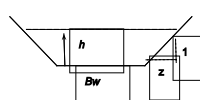
Figure 3.8 Channel Properties
Static hydraulic properties are used to describe the properties of each
channel reach, with each being assumed trapezoidal and include bottom
width (\(B_w`\)), channel length (\(dx\)), channel top width before bankfull
(\(Tw\)), Manning’s roughness coefficient (\(n\)), channel side slope (\(z\),
in meters), and the longitudinal slope of the channel (\(So\)). If a user
is running the model with reach-based routing (channel_option =
1 or 2), the \(B_w\) , \(n\), and \(z\) parameters can be modified
through the Route_Link.nc file. Note: the CHANPARM.TBL
file will not be used in this configuration.
Simulated state variables include estimate of mean water depth in the channel (\(h\)), steady-state velocity (\(v\)) and flow rate (\(q\)) in the reach at the current timestep. An initial depth estimate is made based on the depth from the previous time step. Time varying properties include the hydraulic area, \(Area = (B_w*h*z)*h; (3.23)\), the wetted perimeter \(W_p= (B_w + 2 * \sqrt{1+z^2}); (3.24)\), and the hydraulic radius, \(R=Area/W_p; (3.25)\). With an initial estimate of water depth in the channel, the wave celerity for the trapezoidal channel is estimated as:
Wave celerity is used to estimate the MC routing parameters, where K= dx/ck (3.27) is the time required for an incremental flood wave to propagate through the channel reach, and the storage shape weighting factor is given as, X = \(\frac{1}{2}\left( 1 - \frac{Q}{(Tw{\ c}_{k}\ So\ dx} \right)\) , (3.28) where Q is the estimated discharge, Tw is the water surface width, So is the channel slope and dx is the channel length.
Relevant domain and parameter files/variables:
TOPOGRAPHYin Fulldom_hires.nc - Terrain grid or Digital Elevation Model (DEM). Note: this grid may be provided at resolutions equal to or finer than the native land model resolution.CHANNELGRIDin Fulldom_hires.nc - Channel network grid identifying the location of stream channel grid cellsSTREAMORDERin Fulldom_hires.nc - Strahler stream order grid identifying the stream order for all channel pixels within the channel network.FLOWDIRECTIONin Fulldom_hires.nc - Flow direction grid, which explicitly defines flow directions along the channel network in gridded routing. This variable dictates where water flows into channels from the land surface as well as in the channel. This should not be modified independently because it is tied to the DEM.frxst_pts(optional) in Fulldom_hires.nc - Forecast point grid, which specified selected channel pixels for which channel discharge and flow depth are to be output within a netcdf point file (CHANOBS) and/or an ASCII timeseries file (frxstpts_out.txt).CHANPARM.TBL text or Route_Link.nc netcdf file - Specifies channel parameters by stream order (CHANPARM.TBL, for gridded channel routing) or individual reaches (
route_link_f, for reach-based routing methods)
Note
Reach-based routing is highly sensitive to time step.
3.6.3 Compound Channel (limited configuration)
In order to represent a simplification of the behavior of a flood wave
when it exceeds the channel bank, a compound channel formulation was
added to WRF-Hydro. This option is currently only available when
channel_option=2 and udmp=1 (so using user-defined mapping with
the Muskingum-Cunge reach-based channel routing scheme).
A visual representation is shown in Figure 3.9. When the depth of the
flow exceeds bankfull (\(d > d_b\)), then the wave celerity is given
as the weighted celerity of the trapezoidal flow and the overbank
portion of flow. This weighting is based on the cross-sectional area of
each, and allows water to enter the conceptual compound channel, where
the Manning’s coefficient of the compound channel portion, \(n_{cc}\),
is assumed rougher than the channel \(n\) by an unknown factor,
\(n_{cc}\). Based on a set of sensitivity experiments described in
Read et al., (2023), the default value is
\(n_{cc}=2n\), such that the floodplain roughness is twice that of
the channel. The introduction of compound channel requires values for
three more parameters: bankfull depth (\(d_b\)), top widths of the
trapezoid and the compound channel, \(T_w\) and \(T_{w\_cc},\)
respectively. These parameters, in addition to \(n_{cc}\), are defined
in the Route_Link.nc file. The default values were
determined using a published equation from
Blackburn-Lynch et al., 2017, who gathered regional USGS estimations of
channel parameters and developed coefficients to describe the
relationship of drainage area (\(DA\)) to \(T_w\) and to channel area
(\(A\)). The aggregated CONUS equation is: \(T_w = 2.44(DA)^{0.34}\)
and \(A = 0.75(DA)^{0.53}\). Given these, \(d_b\) is determined
using the standard equation for a trapezoid. As a default value,
\(T_{w\_cc}\) is a multiplier on \(T_w\). Sensitivity experiments
presented in Read et al. (2023) found that \(T_{w\_cc}=3*T_w\)
yielded the best streamflow performance, all else being equal.

Figure 3.9 Cross-sectional schematic of trapezoidal channel and compound channel in National Water Model, where the dashed lines represent roughness of the channel n, and of the compound channel, \(n_{cc}\)
Note
The compound channel option is currently only available when
channel_option=2 and udmp=1 (so using user-defined mapping with
the Muskingum-Cunge reach-based channel routing scheme).
3.7 Lake and Reservoir Routing Description
A simple mass balance, level-pool lake/reservoir routing module allows for an estimate of the inline impact of small and large reservoirs on hydrologic response. A lake/reservoir or series of lakes/reservoirs are identified in the channel routing network, and lake/reservoir storage and outflow are estimated using a level-pool routing scheme. The only conceptual difference between lakes and reservoirs as represented in WRF-Hydro is that reservoirs contain both orifice and weir outlets for reservoir discharge while lakes only contain weirs. Note that the user must adjust these parameters accordingly - the model makes no other distinction between a reservoir and a lake.
Fluxes into a lake/reservoir object occur through the channel network and when surface overland flow intersects a lake object (in the gridded channel routing configuration only). Fluxes from lake/reservoir objects are made only through the channel network and no fluxes from lake/reservoir objects to the atmosphere or the land surface are currently represented (i.e. there is currently no lake evaporation or subsurface exchange between the land surface and lakes and reservoirs). The Level Pool scheme tracks water elevation changes over time, \(h(t)\) where water from the reservoir can exit either through weir overflow (\(Q_w\)) and/or a gate-controlled flow (\(Q_o\)), where these outflows are functions of the water elevation and spillway parameters. Weir flow is given as \(Q_w(t) = C_wLh^{\frac{3}{2}}; (3.29)\) when \(h>h_{max}\) or \(Q_w(t) = 0.0\) when \(h≤h_{max}\) where, \(h_{max}\) is the maximum height before the weir begins to spill (\(m\)), \(C_w\) is a weir coefficient, and \(L\) is the length of the weir (\(m\)). Orifice flow is given as \(Q_o(t) = C_oO_a\sqrt{2gh}; (3.30)\) where \(C_o\) is the orifice coefficient, \(O_a\) is the orifice area (\(m^2\)), and \(g\) is the acceleration of gravity (\(m/s^2\)). In addition, the level pool scheme is designed to track each reservoir’s surface area, \(S_a\) (\(km^2\)) as a function of water depth and the area at full storage, \(A_s\) (\(km^2\)). Presently, a lake/reservoir object is assumed to have vertical side walls, such that the surface area is always constant.

Figure 3.10 Schematic of Level Pool Routing
The lake/reservoir parameters listed below are required for level-pool routing and are defined in the LAKEPARM.nc parameter file. The GIS pre-processing tool can make this file and the model will read it as specified in the hydro.namelist file.
Weir and Orifice Coefficients, \(Cw\), \(Co\) in equations above or
WeirC,OrificeCin LAKEPARM.ncWeir Length (\(m\)), \(L\) in equations above or
WeirLin LAKEPARM.ncWeir Elevation (\(m\)),
WeirEin LAKEPARM.ncOrifice Area (\(m^2\)), \(O_a\) in equations above or
OrificeAin LAKEPARM.ncOrifice Elevation (\(m\)),
OrificeEin LAKEPARM.ncReservoir Area (\(km^2\)), \(A_s\) in equations above or
LkAreain LAKEPARM.ncMaximum reservoir height at full storage (\(m\)), \(h_{max}\) in equations above or
LkMxEin LAKEPARM.ncDam length specified as a multiplier on weir length (\(dimensionless\)), \(Dam_Length\) in LAKEPARM.nc
For the gridded channel routing option, the lake/reservoir routing options
require lake objects to be defined and properly indexed as a data
field in the high resolution terrain routing Fulldom_hires.nc
file. If lake/reservoir objects are present in the
lake grid (and also within the channel network) then level-pool routing through
those objects will occur if CHANRTSWCRT = 1 (channel is active), channel_option
= 3 (gridded routing), and lake_option = 1 (level pool) in hydro.namelist.
For reach-based channel routing options, the lake/reservoir routing options
require lake objects to be defined and properly indexed as waterbody objects
in the Route_Link.nc file.
If lake/reservoir objects are present in the
Route_Link.nc file then level-pool routing through
those objects will occur if CHANRTSWCRT = 1 (channel is active), channel_option
= 1 or 2 (reach routing), and lake_option = 1 (level pool) in hydro.namelist.
The lake_option in hydro.namelist can also be used to turn off lake/reservoir
routing completely (lake_option = 0), set the waterbodies to simply pass water through
from inflow to outflow with no storage or delay (lake_option = 2), or activate data
assimilation (specific to the NOAA National Water Model and not currently
supported outside of that configuration).
There are several special requirements for the lake and channel files when lakes/reservoirs are to be represented and these are discussed in Sections 5.4 and 5.6.
Relevant code modules:
Routing/module_channel_routing.F90
Routing/Reservoirs/Level_Pool/module_levelpool.F90
Relevant namelist options:
hydro.namelist:
lake_option- Option to specify lake/reservoir routing behavior (0=lakes off, 1=level pool, 2=passthrough, 3=reservoir DA).route_lake_f- Path to lake parameter file to support level-pool reservoir routing methods.
Note
As mentioned in the paragraph above, if in the
GIS-Preprocessing the user created a “gridded” routing stack for
channel_option = 3 (i.e. did not select to create a
Route_Link.nc file for channel_option=1 or =2) AND specified
a lake file (user provided a reservoir/lake input file), then
the Fulldom_hires.nc file will populate the LAKEGRID variable.
For this case, the user must specify the route_lake_f file.
To turn lakes “off” with channel_option=3, create another set
of Fulldom_hires.nc (“domain”) files without a reservoir input
file specified.
Relevant domain and parameter files/variables:
CHANNELGRIDin Fulldom_hires.nc - Channel network grid identifying the location of stream channel grid cellsLAKEGRIDin Fulldom_hires.nc (optional) - Specifies lake locations on the channel grid (for gridded channel routing methods, i.e.channel_option=3).Route_Link.nc netCDF file (optional) - Specifies lake associations with channel reaches.
LAKEPARM.nc netCDF file - Specifies lake parameters for each lake object specified.
3.8 Conceptual base flow model description
Aquifer processes contributing baseflow often operate at depths well below ground surface. As such, there are often conceptual shortcomings in current land surface models in their representation of groundwater processes. Because these processes contribute to streamflow (typically as “baseflow”) a parameterization is often used in order to simulate total streamflow values that are comparable with observed streamflow from gauging stations. Therefore, a switch-activated baseflow module Routing/module_GW_baseflow.F90 has been created which conceptually (i.e. not physically-explicit) represents baseflow contributions to streamflow. This model option is particularly useful when WRF-Hydro is used for long-term streamflow simulation/prediction and baseflow or “low flow” processes must be properly accounted for. Besides potential calibration of the land surface model parameters the conceptual baseflow model does not directly impact the performance of the land surface model scheme. The new baseflow module is linked to WRF-Hydro through the discharge of “deep drainage” from the land surface soil column (sometimes referred to as “underground runoff”).
The baseflow parameterization in WRF-Hydro uses spatially-aggregated drainage from the soil profile as recharge to a conceptual groundwater reservoir (Fig. 3.10). The unit of spatial aggregation is often taken to be that of a catchment or sub-basin within a watershed. Each sub-basin has a groundwater reservoir “bucket” with a conceptual depth and associated conceptual volumetric capacity. The reservoir operates as a simple bucket where outflow (= “baseflow” or “stream inflow”) is estimated using an empirically-derived function of recharge. The functional type and parameters are determined empirically from offline tests using an estimation of baseflow from stream gauge observations and model-derived estimates of bucket recharge provided by WRF-Hydro. Presently, WRF-Hydro uses either a direct output-equals-input (“pass-through”) relationship or an exponential storage-discharge function for estimating the bucket discharge as a function of a conceptual depth of water in the bucket (“exponential bucket”). Note that, because this is a highly conceptualized formulation, the depth of water in the bucket in no way infers the actual depth of water in a real aquifer system. However, the volume of water that exists in the bucket needs to be tracked in order to maintain mass conservation. Estimated baseflow discharged from the bucket model is then combined with lateral inflow from overland routing (if active) and input directly into the stream network as channel inflow, as referred to above in Section 3.5. Presently, the total basin baseflow flux to the stream network is equally distributed among all channel pixels within a basin for gridded channel routing options or dumped into the top of the reach to be routed downstream for reach-based methods. Lacking more specific information on regional groundwater basins, the groundwater/baseflow basins in WRF-Hydro are often assumed to match those of the surface topography. However, this is not a strict requirement. Buckets can be derived in a number of ways such as where true aquifers are defined or from a third-party hydrographic dataset such as the USGS NHDPlus or Hydrosheds.
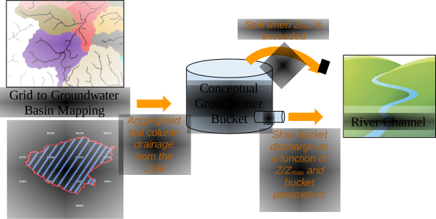
Figure 3.11 Hypothetical map of groundwater/baseflow sub-basins within a watershed and conceptualization of baseflow “bucket” parameterization in WRF-Hydro.
- \(z = z_{previous} + \frac{Q_{in}*dt}{A}; \qquad (3.40)\)if \(z > z_{max}\) :\(z_{spill} = z - z_{max}\)\(z = z_{max}\)\(Q_{spill} = \frac{A*z_{spill}}{dt}\)else :\(Q_{spill} = 0\)\(Q_{exp} = C(e^{E\frac{z}{zmax}}-1)\)\(Q_{out} = Q_{spill} + Q_{exp}\)\(z = z - \frac{Q_{exp}*dt}{A}\)where :\(Q_{in}\) is the inflow to the bucket aggregated from the bottom of the LSM in \(m^3/s\)\(z\) is the height of the water level in the bucket in \(mm\)\(z_{max}\) is the total height of the bucket in \(mm\)\(A\) is the area of the catchment or groundwater basin in \(m^2\)\(E\) is a unitless parameter\(C\) is a parameter with units of \(m^3/s\)
A groundwater/baseflow bucket model parameter file (GWBUCKPARM.nc) specifies the empirical parameters governing the behavior of the bucket model parameterization for each groundwater/baseflow basin specified within the model domain. These files are created by the WRF-Hydro GIS Preprocessing System and documented in Appendix 10. The parameters include: the bucket model coefficient, the bucket model exponent, the initial depth of water in the bucket model, and the maximum storage in the bucket before “spilling” occurs.
It is important to remember that a simple bucket model is a highly abstracted and conceptualized representation of groundwater processes and therefore the depth of water values in the bucket and the parameters themselves have no real physical basis. As mentioned above, initial values of the groundwater bucket model parameters are typically derived analytically or 'offline' from WRF-Hydro and then are fine-tuned through model calibration.
There are 4 options available for the conceptual baseflow model, as specified
in GWBASESWCRT in hydro.namelist. The conceptual baseflow model
can be turned off (GWBASESWCRT = 0), which means water draining from the soil column in the land
surface model will become a sink term (this water will not be returned to the channel
and will be a loss from the system). The exponential bucket model can be activated
(GWBASESWCRT = 1), as described above. Water draining from the land model soil
column can be placed directly into the channel with no additional storage/attenuation
(GWBASESWCRT = 2). For configurations using user-defined mapping to specify
catchment boundaries (UDMP_OPT = 1), there is a modified version of the
exponential bucket model (GWBASESWCRT = 4) that adjusts the \(C\) parameter above
based on the area of the catchment.
Relevant code modules:
Routing/module_GW_baseflow.F90
Relevant namelist options:
hydro.namelist:
GWBASESWCRT- Switch to activate groundwater bucket module.GWBUCKPARM_file- Path to groundwater bucket parameter file.gwbasmskfil(optional) - Path to netcdf groundwater basin mask file if using an explicit groundwater basin 2d grid.UDMP_OPT(optional) - Switch to activate user-defined mapping between land surface model grid and conceptual basins.udmap_file(optional) - If user-defined mapping is active, path to spatial-weights file.
Relevant domain and parameter files/variables:
GWBUCKPARM.nc netCDF file - Specifies the parameters for each groundwater bucket/basin. More information regarding the groundwater bucket model parameters is provided in Section 5.5 and Appendix 10.
GWBASINS.nc netCDF file - The 2d grid of groundwater basin IDs.
spatialweights.nc - netCDF file specifying the weights to map between the land surface grid and the pre-defined groundwater basin boundaries.